 Z. Michael Gehlke
Effective Semantics: Shape Types Have Operations
Abstract
This paper is the second in our series on effective semantics, working on introducing the concept of digital images as an encoding for shape types.
In this paper, we’ll be building on the correspondence introduced in our first paper to explore how we can encode shape operations in a general way. In the simple cases of iterated interval and loop products, we can do them by hand – but what correctly generalizes these operations for more complex shapes?
We’ll introduce three operations:
- addition between two shapes;
- multiplication of one shape by another; and,
- iterated multiplication.
Together with the gluing operation between cells in a shape (introduced last paper in the constructions), these will allow for the building of complex models. At each step along the way, we’ll see how these operations work on both points (replicating arithmetic) and simple shapes, such as the interval.
Readers may want to browse the following code while reading:
Familiar Shape Types
These types are initially introduced in our first paper, and we briefly cover their encoding into digital images to refresh the reader. We add the torus to the collection of 2D shapes.
0-Dimension
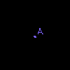
We can recall that there is a single type of dimension 0, which is the Point type representing a single datum.
We represent that same object in four ways: as a term; as a decorated geometric object; as a construction diagram; and as a digital image. As before, in all of the digital images, purple pixels represent an equality map; pink pixels represent an inclusion map; and blue pixels represent a restriction map.
| Type | Shape | Diagram | Image |
|---|---|---|---|
Point(a) |
 |
 |
 |
1-Dimension
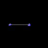
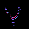
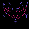
We can further recall the two main geometric types for 1-dimension, the Interval and the Loop – with the chief distinction being that the Loop is an Interval where 0=1.
| Type | Shape | Diagram | Image |
|---|---|---|---|
Interval(a, b) |
 |
 |
 |
Loop(a, b, a=b) |
 |
 |
 |
2-Dimension
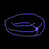
For the 2-dimension types, we’ll include the two from before (Cylinder and Square) with a new type, the Torus. Together, these three will form the products of Interval and Loop.
| Type | Shape | Diagram | Image |
|---|---|---|---|
Cylinder(...) |
 |
 |
 |
Square(...) |
 |
 |
 |
Familiar Shape Relationships
The following examples are relationships that will be familiar to many readers and guide our intuition in defining the product of shape types.
For each of them, we represent the relationship in the four ways above, but stacked vertically. This helps see the relationship between them.
A Square is a Product of Intervals
Here we view the product of intervals through shape, diagram, and digital image perspectives.
Interval |
x | Interval |
= | Square |
|---|---|---|---|---|
|
|
|
||
|
|
|
||
|
|
|
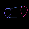
A Cylinder is a Product of an Interval and a Loop
Here we view the product of an interval and loop through shape, diagram, and digital image perspectives.
Interval |
x | Loop |
= | Cylinder |
|---|---|---|---|---|
|
|
|
||
|
|
|
||
|
|
|
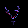
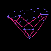
A Torus is a Product of Loops
Here we view the product of loops through shape, diagram, and digital image perspectives.
Loop |
x | Loop |
= | Torus |
|---|---|---|---|---|
|
|
 |
||
|
|
 |
||
|
|
 |
Defining Shape Type Operations as Image Transforms
We want to define the product on shapes encoded as digital images. To do this, we will first define addition on shapes. Then multiplication will be defined as modified iterated-addition. We will also add a scalar exponentiation, such as in Cube = Interval ** n.
Definition 1: Shape + Shape
The most basic example is to add two shapes without any additional structure: one apple sitting next to another apple.
This can be encoded in digital images in a fairly basic way:
A + B = [[A,0], [0,B]]
This creates a new image, with one shape in the upper left and one shape in the lower right. In the case of addition, there is no structure created between these two shapes – though in the case you were building a gluing from the addition, these “flanks” are where you’d add the equivalences to “glue” the two shapes together.
In the case of point objects, this behavior replicates the familiar 2 + 3 = 5:
2 |
+ | 3 |
= | 5 |
|---|---|---|---|---|
 |
 |
 |
Definition 2: Shape * Shape
The next operation, however, is more complicated: one shape “applied” to the other.
This is best though of as two steps –
The first to create a copy of R-operand for each object in the L-operand:
A *' B = [[B,0,...,0], [0,B,...,0], ..., [0,0,...,B]]
In the case of point objects, this behavior replicates the familiar 2 * 3 = 6:
2 |
* | 3 |
= | 6 |
|---|---|---|---|---|
|
|
 |
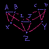
The second step the “attaches” these copies of the R-operand object-wise, based on the structure of the L-operand:
A * B = [[B, a_12 * I, a_13 * I, ..., a_1n * I], ..., [a_n1 * I, a_n2 * I, a_n3 * I, ..., a_n(n-1) * I, B]]
This has no analog in familiar arithmetic, as numbers are emulated by disjoint point objects. However, we can see it in the product of intervals (repeated from above). We can see that along the diagonal, there are three copies of the original 3x3 Interval image – with connections between those blocks.
Interval |
x | Interval |
= | Square |
|---|---|---|---|---|
|
|
|
Definition 3: Shape ** n
The final operation is simple: iterated multiplication.
This can be thought of as S ** n = S * S * ... * S in more or less the standard way to define natural exponentiation. This concept can reasonably be extended to include n=0 by defining that to be the Point object.
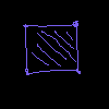
And when applied to the interval, we get the expected sequence:
| Interval ** n | Image |
|---|---|
| 0 |  |
| 1 |  |
| 2 |  |
| 3 | 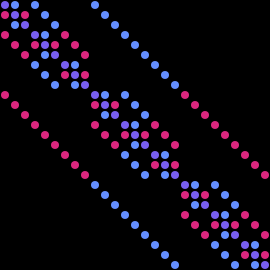 |
| 4 | 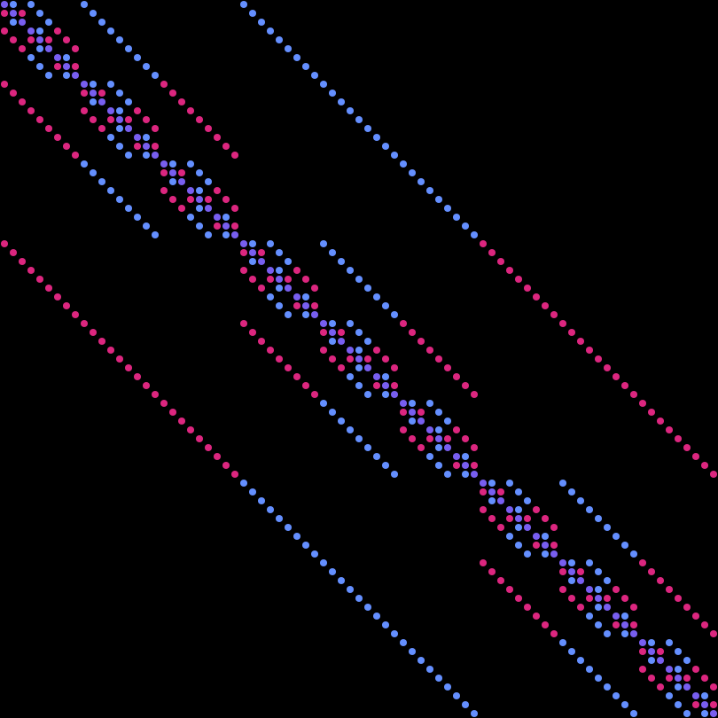 |
Conclusions
Shape types can be modeled as digital images and this paper explored how operations on shapes are transforms on their digital image projection. This shows that the mapping from shapes to digital images not only accurately represents the shapes themselves, but the operations on them as well. This is key to using digital image encodings as a method of fast mathematical reasoning: we can perform our mathematical operations entirely encoded as digital images!
We saw this mapping in two ways:
- that operations on points reproduce the arithmetic we’re expecting, and
- that operations on products produce the higher-order structures we expect.
We hope that you found this introduction to operating on shapes via digital image projections useful.
Future Work
This paper is the second in our series on digital images as an encoding for mathematical reasoning. We will be continuing this work in two ways:
- by exploring the division operation on shapes in an upcoming paper; and,
- by exploring how we can model groups using digital image encodings.